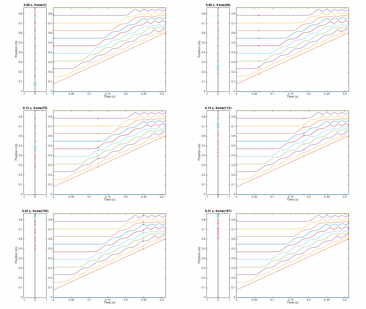
I used animation to help me visualize some of the work I did for my honours thesis (PDF warning). Prior to MATLAB R2014b’s major graphics changes, it wasn’t exactly easy to create efficient animations with MATLAB, so I spent some time figuring out the best way to do it.
This is what I had in the end:

The “easy” way
Say you want to animate a particle trajectory (position vs time), the most obvious way would be to use plot() in a for loop, kind of like this:
% Animation loop
for i = 1:totalFrames
  % Compute the necessary data
  particlePosition(i) = rand;

  % Plot the result of the computation
  plot(timeFrame(i), particlePosition(i));
end
If you’ve ever tried doing this you would notice that it does not scale well. Even if the plot is just a little bit complex this method becomes very slow, with lots of flashes of the figure window. Every time plot() is called MATLAB has to repeat a lot of unnecessary work.1
A better method
In MathWorks’ article on animation techniques, we can see that they recommend
Update the properties of a graphics object and display the updates on the screen. This technique is useful for creating animations when most of the graph remains the same. For example, set the
XDataandYDataproperties repeatedly to move an object in the graph.
Instead of using plot(), the set() function skips a lot of unnecessary work, making it more efficient. An implementation example would look like this:
% Initialize the plot
h = plot(timeFrame(1), particlePosition(1));

% Animation loop
for i = 2:totalFrames
    % Compute the necessary data
  particlePosition(i) = rand;

  % Change the data in the plot
  set(h, 'XData', timeFrame(i));
  set(h, 'YData', particlePosition(i));
end
Note: Sometimes, especially if your animation update command is after complicated computation, you need to use drawnow to force the animation to occur in real time.
A quick example
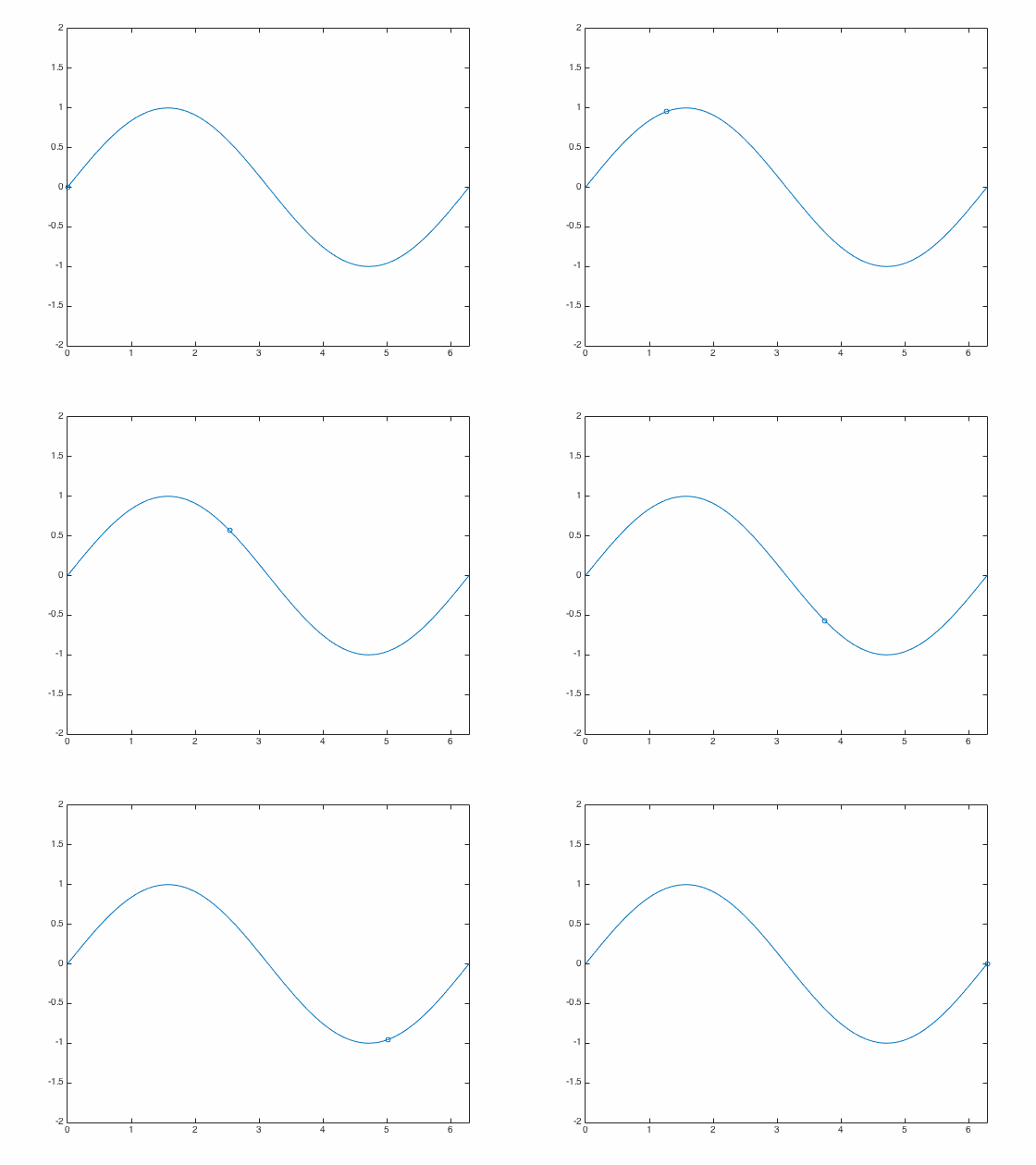
I wrote a simple script that uses this technique to animate a particle in a sine trajectory. It should look like this:2

Full source:
| N = 100; | |
| x = linspace(0,2*pi,N); | |
| y = sin(x); | |
| %% Initialization | |
| % set up first frame | |
| figure('Color', 'white'); | |
| % plot the 'background' | |
| plot(x, y, 'LineWidth', 1); | |
| % set up the markers that move | |
| h = line(x(1),y(1),'Marker', 'o', 'MarkerSize', 5); | |
| % set up axes size | |
| xlim([0 2*pi]); | |
| ylim([-2 2]); | |
| % get figure size | |
| pos = get(gcf, 'Position'); | |
| width = pos(3); height = pos(4); | |
| % preallocate data (for storing frame data) | |
| mov = zeros(height, width, 1, length(N), 'uint8'); | |
| %% Method 1: update XData and YData | |
| for i = 1:N | |
| set(h, 'XData', x(i)); | |
| set(h, 'YData', y(i)); | |
| drawnow update | |
| % get frame as an image | |
| f = getframe(gcf); | |
| % create a colormap for the first frame. For the rest of the frames, | |
| % use the same colormap | |
| if i == 1 | |
| [mov(:,:,1,i), map] = rgb2ind(f.cdata, 256, 'nodither'); | |
| else | |
| mov(:,:,1,i) = rgb2ind(f.cdata, map, 'nodither'); | |
| end | |
| end | |
| % Create animated GIF | |
| imwrite(mov, map, 'animation.gif', 'DelayTime', 1/60, 'LoopCount', inf); | |
| %% | |
| % *Animated GIF* | |
| % | |
| % <<../animation.gif>> |
Animating multiple trajectories
I ran into some problems when I needed to animate variable number of trajectories. I wanted to visualize how changing the number of particles in my system changed the trajectories, but MATLAB was giving me errors when I used the set() method.
It turns out that animating multiple trajectories in stored one variable3 with the same time vector requires a trick. The old method won’t work if the number of trajectories will be changing all the time. I will illustrate with an example:
% Initialize the trajectories
particlePosition = zeros(randi(5),totalFrames)

% Initialize the plot
h = plot(timeFrame(1), particlePosition(:,1));

% Animation loop
for i = 2:totalFrames
  % Compute the necessary data
  for j = 1:size(particlePosition,1)
    particlePosition(j,i) = rand;
  end

  % Change the data in the plot
  set(h, 'XData', timeFrame(i));
  set(h, {'YData'}, num2cell(particlePosition(:,i)));
end
Here, particlePosition contains up to five trajectories. Note the use of num2cell in setting YData is required for the animation to work properly because of the way graphics data are structured in MATLAB.
Note: TheYData you are setting must be a column cell vector. So if your data is structured such that each row represents a frame in the animation, you must transpose your data in set().
Another quick example
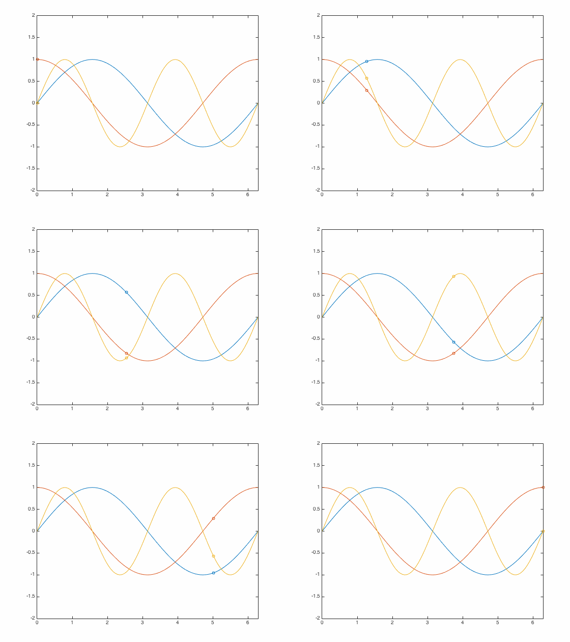
You can download the other script to see how this can be implemented. It looks like this:

Full source:
| clear all | |
| N = 100; | |
| x = linspace(0,2*pi,N); | |
| % Make 3 different paths | |
| y(1,:) = sin(x); | |
| y(2,:) = cos(x); | |
| y(3,:) = sin(2*x); | |
| %% Initialization | |
| % set up first frame | |
| figure('Color', 'white'); | |
| % plot the 'background' | |
| plot(x, y, 'LineWidth', 1); | |
| % set up the markers that move | |
| h = line(x(1),y(:,1),'Marker', 'o', 'MarkerSize', 5); | |
| % set up axes size | |
| xlim([0 2*pi]); | |
| ylim([-2 2]); | |
| % get figure size | |
| pos = get(gcf, 'Position'); | |
| width = pos(3); height = pos(4); | |
| % preallocate data (for storing frame data) | |
| mov = zeros(height, width, 1, length(N), 'uint8'); | |
| %% Animation loop with update method | |
| for i = 1:N | |
| set(h, 'XData', x(i)); | |
| set(h, {'YData'}, num2cell(y(:, i))); | |
| % get frame as an image | |
| f = getframe(gcf); | |
| % create a colormap for the first frame. For the rest of the frames, | |
| % use the same colormap | |
| if i == 1 | |
| [mov(:,:,1,i), map] = rgb2ind(f.cdata, 256, 'nodither'); | |
| else | |
| mov(:,:,1,i) = rgb2ind(f.cdata, map, 'nodither'); | |
| end | |
| end | |
| % Create animated GIF | |
| imwrite(mov, map, 'animation.gif', 'DelayTime', 1/60, 'LoopCount', inf); | |
| %% | |
| % *Animated GIF* | |
| % | |
| % <<../animation.gif>> |
An example from MathWorks
I learned a lot from MathWorks’ animation example here: https://www.mathworks.com/examples/matlab/4020-animation, including how to export as GIFs.